Use sitePath to find fixation and parallel sites
Chengyang Ji
Source:vignettes/sitePath.Rmd
sitePath.RmdAbstract
In viral evolution, fixed substitutions in the nucleic acid or protein level are closely associated with maintaining viral function, while parallel mutation reflects the competitive nature in adaptive selection. The continued accumulation of large-scale viral sequence data enhances the challenge of identifying important mutations in a quick and accurate manner. In sitePath, the phylogenetic tree was separated into a set of inheritable phylogenetic pathways via an automated pathway-division method. Then, for each phylogenetic pathway, the identification of fixed substitutions was transformed into a local-optimal-solution problem directed by a minimal entropy algorithm. Finally, the parallel mutation was determined based on the recurrence of mutations among at least two phylogenetic pathways.
Introduction
The sitePath package is made for the high-throughput
identification of fixed substitutions and parallel mutations in viruses
from a single phylogenetic tree. This is achieved by three major
steps:
- Clustering phylogenetic terminals
- Identifying phylogenetic pathways
- Finding fixed and parallel mutations
Clustering phylogenetic terminals
The firs step is to import phylogenetic tree and multiple sequence
alignment files. For now, sitePath accepts
phylo object and alignment object. Functions
from ggtree and seqinr are able to handle most
file formats.
Import tree file
The S3 phylo class is a common data structure for
phylogenetic analysis in R. The CRAN package ape
provides basic parsing function for reading tree files. The Bioconductor
package treeio
provides more comprehensive parsing utilities.
library(sitePath)

tree_file <- system.file("extdata", "ZIKV.newick", package = "sitePath")
tree <- read.tree(tree_file)
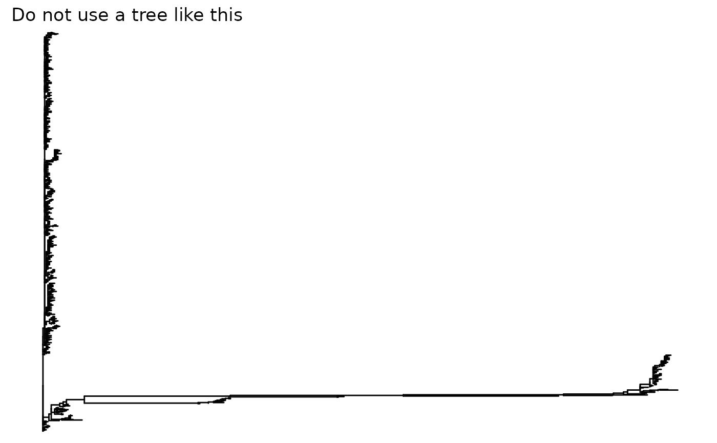
It is highly recommended that the file stores a rooted tree as R would consider the tree is rooted by default and re-rooting the tree in R is difficult. Also, we expect the tree to have no super long branches. A bad example is shown below:
Import sequence alignment file
Most multiple sequence alignment format can be parsed by seqinr.
There is a wrapper function for parsing and adding the sequence
alignment. Set “cl.cores” in options to the number of cores
you want to use for multiprocessing.
alignment_file <- system.file("extdata", "ZIKV.fasta", package = "sitePath")

options(list("cl.cores" = 1)) # Set this bigger than 1 to use multiprocessing

paths <- addMSA(tree, msaPath = alignment_file, msaFormat = "fasta")Identifying phylogenetic pathways
After importing the tree and sequence file, sitePath is
ready to identify phylogenetic pathways.
The impact of threshold on resolving lineages
The impact of threshold depends on the tree topology hence there is
no universal choice. The function sneakPeak samples
thresholds and calculates the resulting number of paths. The use of
this function can help choose the threshold.
preassessment <- sneakPeek(paths, makePlot = TRUE)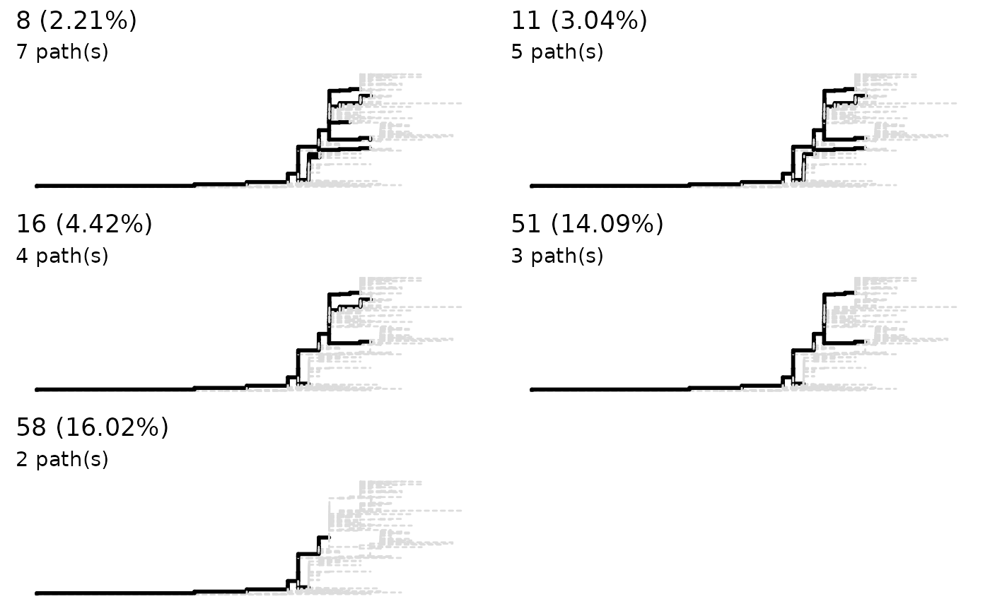
Choose a threshold
The default threshold is the first ‘stable’ value to produce the same
number of phylogenetic pathways. You can directly use the return of
addMSA if you want the default or choose other threshold by
using function lineagePath. The choice of the threshold
really depends. Here 18 is used as an example.
paths <- lineagePath(preassessment, 18)
paths
#> This is a 'lineagePath' object.
#>
#> 4 lineage paths using 18 as "major SNP" threshold
You can visualize the result.
plot(paths)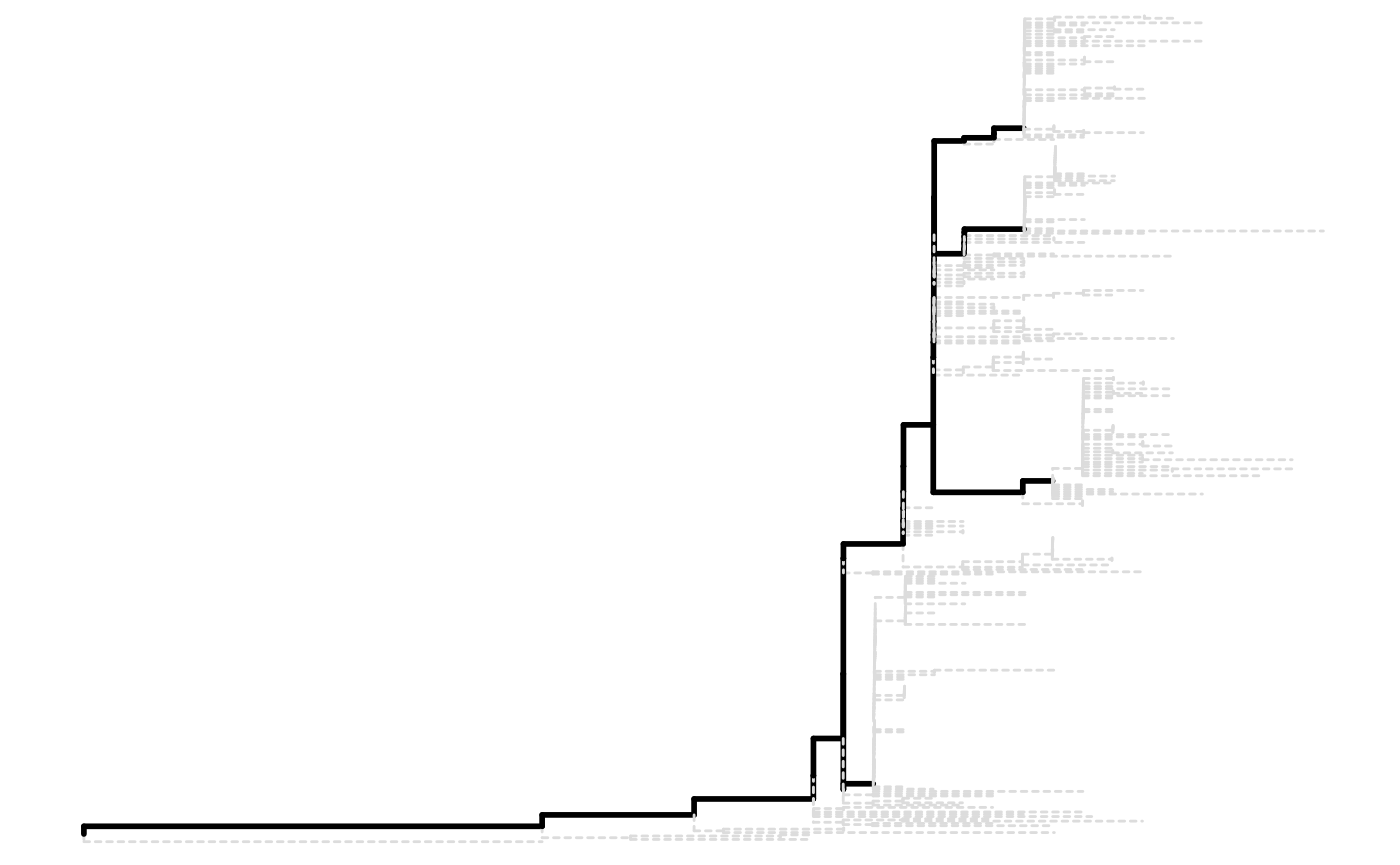
Finding fixed and parallel mutations
Now you’re ready to find fixation and parallel mutations.
Entropy minimization
The sitesMinEntropy function perform entropy
minimization on every site for each lineage. The fixation and parallel
mutations can be derived from the function’s return value.
minEntropy <- sitesMinEntropy(paths)Fixation mutations
The hierarchical search is done by fixationSites
function. The function detects the site with fixation mutation.
fixations <- fixationSites(minEntropy)
fixations
#> This is a 'fixationSites' object.
#>
#> Result for 4 paths:
#>
#> 139 894 2074 2086 2634 3045 988 1143 2842 3398 107 1118 3353
#> No reference sequence specified. Using alignment numbering
To get the position of all the resulting sites,
allSitesName can be used on the return of
fixationSites and also other functions like
SNPsites and parallelSites.
allSites <- allSitesName(fixations)
allSites
#>  [1] "139"  "894"  "2074" "2086" "2634" "3045" "988"  "1143" "2842" "3398"
#> [11] "107"  "1118" "3353"
If you want to retrieve the result of a single site, you can pass the
result of fixationSites and the site index to
extractSite function. The output is a sitePath
object which stores the tip names.
sp <- extractSite(fixations, 139)It is also possible to retrieve the tips involved in the fixation of the site.
extractTips(fixations, 139)
#> [[1]]
#>  [1] "ANK57896" "AMD61711" "AQS26698" "APG56458" "AUI42289" "AMR39834"
#>  [7] "AWH65848" "APO08504" "AMX81917" "AVZ47169" "AMX81916" "AMD61710"
#> [13] "AMK49492" "AMX81915" "AOC50652" "APH11611" "BBC70847" "AUF35022"
#> [19] "ATL14618" "AUF35021" "AVV62004" "BAX00477"
#> attr(,"AA")
#> [1] "S"
#>
#> [[2]]
#>   [1] "BAV89190"     "AOI20067"     "AMM43325"     "AMM43326"     "AUI42329"
#>   [6] "AUI42330"     "ANC90425"     "AMT75536"     "ANF16414"     "AMR68932"
#>  [11] "ANA12599"     "AMM39806"     "AMR39830"     "AMV49165"     "AMO03410"
#>  [16] "ANO46307"     "AVG19275"     "ANN44857"     "ANO46306"     "ANO46309"
#>  [21] "ANO46305"     "ANO46303"     "ARB08102"     "ANO46302"     "AHZ13508"
#>  [26] "ANO46304"     "ANO46301"     "ANO46308"     "AOG18296"     "AOO19564"
#>  [31] "AUI42194"     "APC60215"     "AMQ48986"     "ATG29307"     "ART29828"
#>  [36] "AWF93617"     "ATG29284"     "ATG29287"     "ATG29303"     "AWF93619"
#>  [41] "AWF93618"     "AQM74762"     "AUD54964"     "AQM74761"     "ATG29306"
#>  [46] "ASL68974"     "ATG29267"     "ASL68978"     "AQX32985"     "ATG29315"
#>  [51] "AQZ41956"     "ARI68105"     "ASU55505"     "AQZ41949"     "ASL68979"
#>  [56] "ATG29299"     "ATI21641"     "ATG29270"     "ATG29291"     "AOY08536"
#>  [61] "ANO46297"     "ANO46298"     "AQZ41950"     "AQZ41951"     "ARU07183"
#>  [66] "ANG09399"     "AQZ41954"     "AOY08533"     "AQZ41947"     "AQZ41948"
#>  [71] "ATG29292"     "ATG29295"     "AOW32303"     "AVZ25033"     "AOC50654"
#>  [76] "AQZ41953"     "ATG29301"     "ATG29276"     "APO08503"     "AMC13913"
#>  [81] "AMC13912"     "APO39243"     "APO39229"     "AQZ41952"     "AQZ41955"
#>  [86] "AMK49165"     "ARB07976"     "APB03018"     "AMC13911"     "APB03019"
#>  [91] "ASU55416"     "ANK57897"     "AWH65849"     "AMZ03556"     "ASU55417"
#>  [96] "ANW07476"     "APY24199"     "AMA12086"     "AMH87239"     "APY24198"
#> [101] "APO36913"     "ALX35659"     "AOG18295"     "ANQ92019"     "AML81028"
#> [106] "APY24200"     "AMD16557"     "ARU07074"     "AOX49264"     "AOX49265"
#> [111] "AOY08518"     "ARB07962"     "AMX81919"     "AMM39805"     "ARX97119"
#> [116] "AMB37295"     "AMK79468"     "AML82110"     "AMR39831"     "AMX81918"
#> [121] "ANC90426"     "ALU33341"     "ASB32509"     "AMA12085"     "AMU04506"
#> [126] "AMA12087"     "AMA12084"     "AQU12485"     "AMS00611"     "AMQ48981"
#> [131] "AOY08538"     "APH11492"     "AOY08517"     "AOY08541"     "AOO54270"
#> [136] "AND01116"     "ARU07076"     "AMK49164"     "APG56457"     "AOR82892"
#> [141] "ATB53752"     "ANH10698"     "AOR82893"     "ARU07075"     "AMB18850"
#> [146] "YP_009428568" "AMQ48982"     "ART29823"     "APW84876"     "ASK51714"
#> [151] "ARB07953"     "APW84872"     "AOY08525"     "APW84873"     "AOY08535"
#> [156] "AVZ25035"     "ARB07932"     "AOY08523"     "AOY08542"     "ASW34087"
#> [161] "AOY08537"     "APB03020"     "ART29826"     "ART29825"     "AOS90220"
#> [166] "AMN14620"     "APW84874"     "APW84875"     "BAV82373"     "AOS90221"
#> [171] "AOS90224"     "APB03021"     "APO39232"     "AOS90223"     "APO39237"
#> [176] "ANH22038"     "APW84877"     "APO39236"     "AOY08546"     "AOY08516"
#> [181] "APO39233"     "AOS90222"     "AOO53981"     "AOY08521"     "AOO85388"
#> [186] "APO39228"     "ARB07967"     "ANF04752"     "AOE22997"     "APQ41782"
#> [191] "APQ41786"     "ASU55393"     "ASU55404"     "ASU55423"     "ANB66182"
#> [196] "ASU55425"     "ASU55420"     "AQX32986"     "ASU55422"     "APQ41784"
#> [201] "ANC90428"     "ASU55415"     "ASU55418"     "ARM59239"     "ASU55408"
#> [206] "ASU55424"     "ASU55390"     "ASU55419"     "ASU55391"     "AMM39804"
#> [211] "ASU55411"     "ANB66183"     "ASU55421"     "AMZ03557"     "ASU55392"
#> [216] "AQX32987"     "ASU55403"     "ASU55399"     "APQ41783"     "ANS60026"
#> [221] "ANB66184"     "ASU55426"     "ASU55412"     "ASU55413"     "ASU55410"
#> [226] "ASU55397"     "ASU55400"     "ASU55409"     "APB03017"     "ASU55395"
#> [231] "ASU55396"     "AOY08524"     "ASU55394"     "ASU55414"     "ASU55405"
#> [236] "AMC33116"     "ASU55406"     "ASU55398"     "ASU55407"     "AMQ34003"
#> [241] "AMQ34004"     "ASU55401"     "ASU55402"
#> attr(,"AA")
#> [1] "N"
Use plot on a sitePath object to visualize
the fixation mutation of a single site. Alternatively, use
plotSingleSite on an fixationSites object with
the site specified.
plot(sp)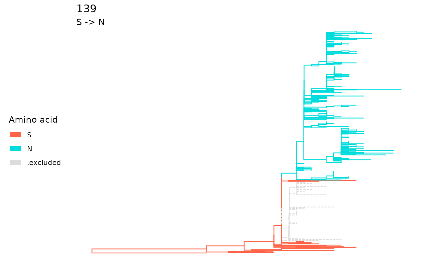
plotSingleSite(fixations, 139)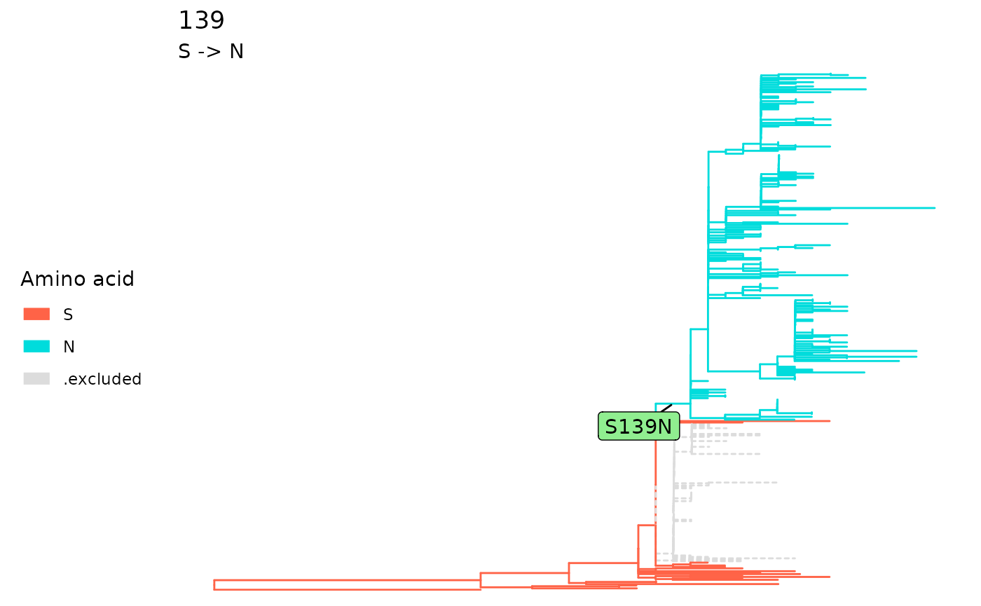
To have an overall view of the transition of fixation mutation:
plot(fixations)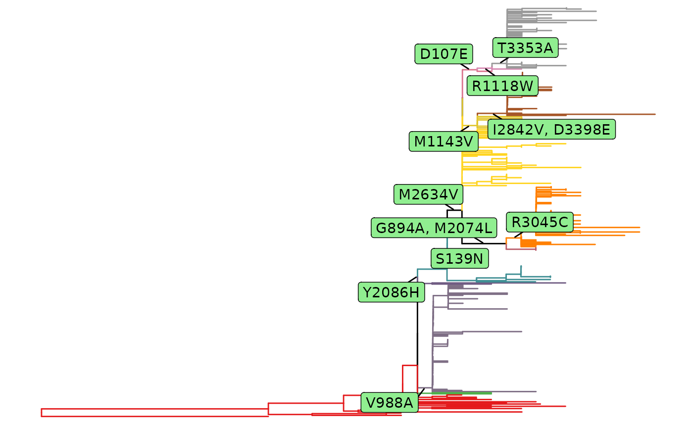
Parallel mutations
Parallel mutation can be found by the parallelSites
function. There are four ways of defining the parallel mutation:
all, exact, pre and
post. Here exact is used as an example.
paraSites <- parallelSites(minEntropy, minSNP = 1, mutMode = "exact")
paraSites
#> This is a 'parallelSites' object.
#>
#> Result for 4 paths:
#>
#> 105 1264 1226 1717 988 2611 2787 2749 3328 3162 1857 3046 1016 1171 1327 3076 106 2357 573 1404 940 1180
#> No reference sequence specified. Using alignment numbering
The result of a single site can be visualized by
plotSingleSite function.
plotSingleSite(paraSites, 105)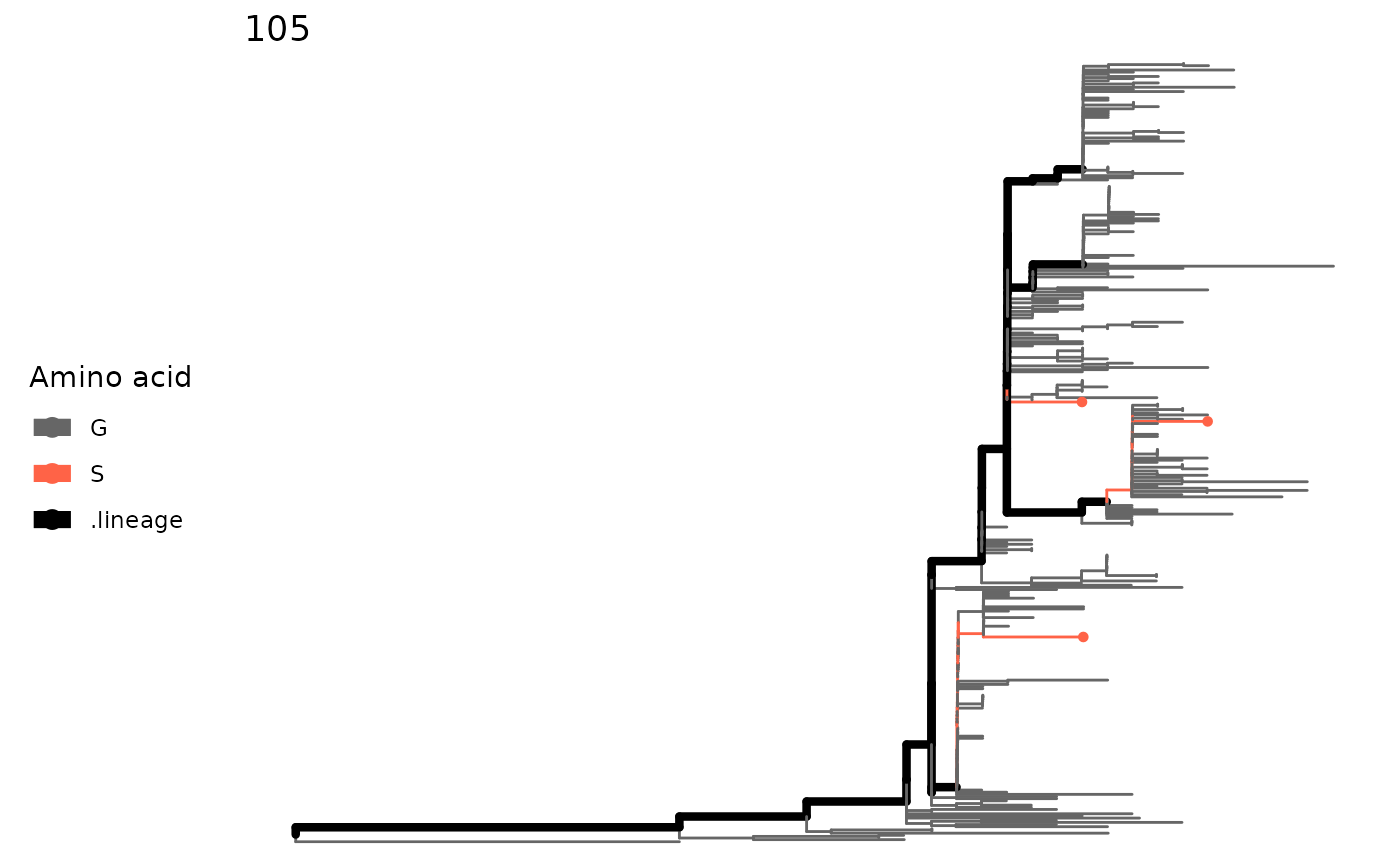
To have an overall view of the parallel mutations:
plot(paraSites)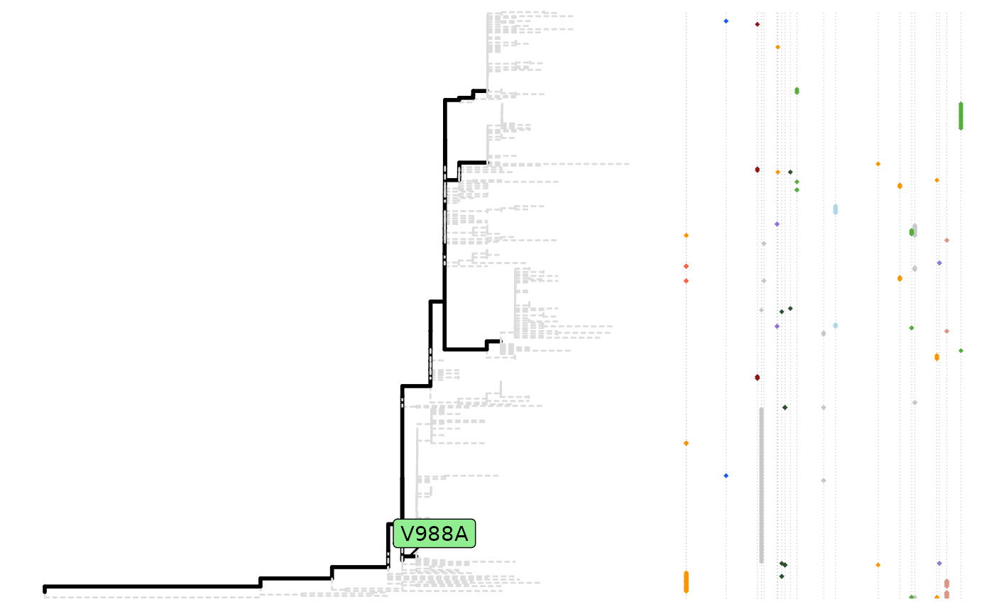
Miscellaneous
This part is extra and experimental but might be useful when pre-assessing your data. We’ll use an example to demonstrate.
Inspect one site
The plotSingleSite function will color the tree
according to amino acids if you use the output of
lineagePath function.
plotSingleSite(paths, 139)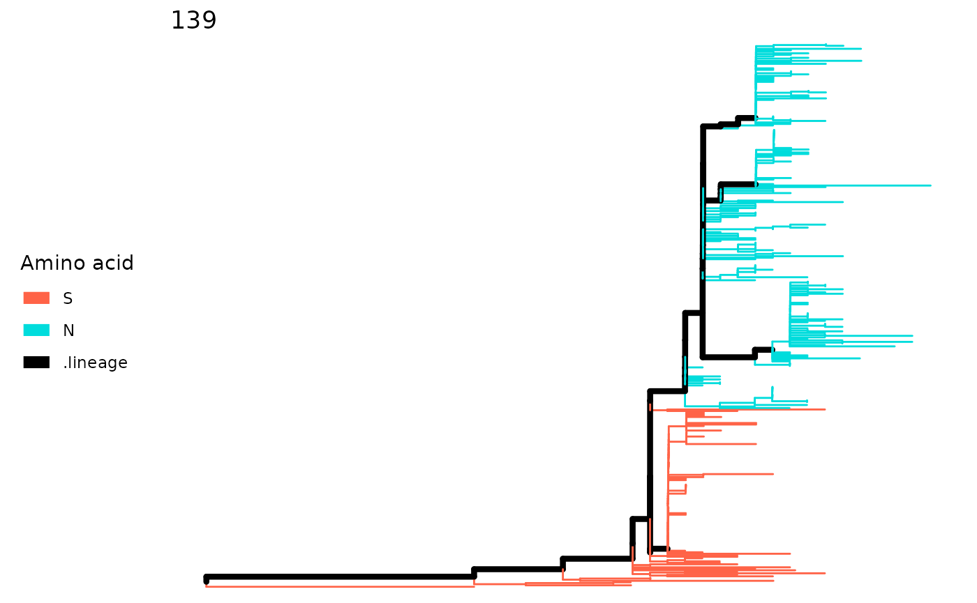
plotSingleSite(paths, 763)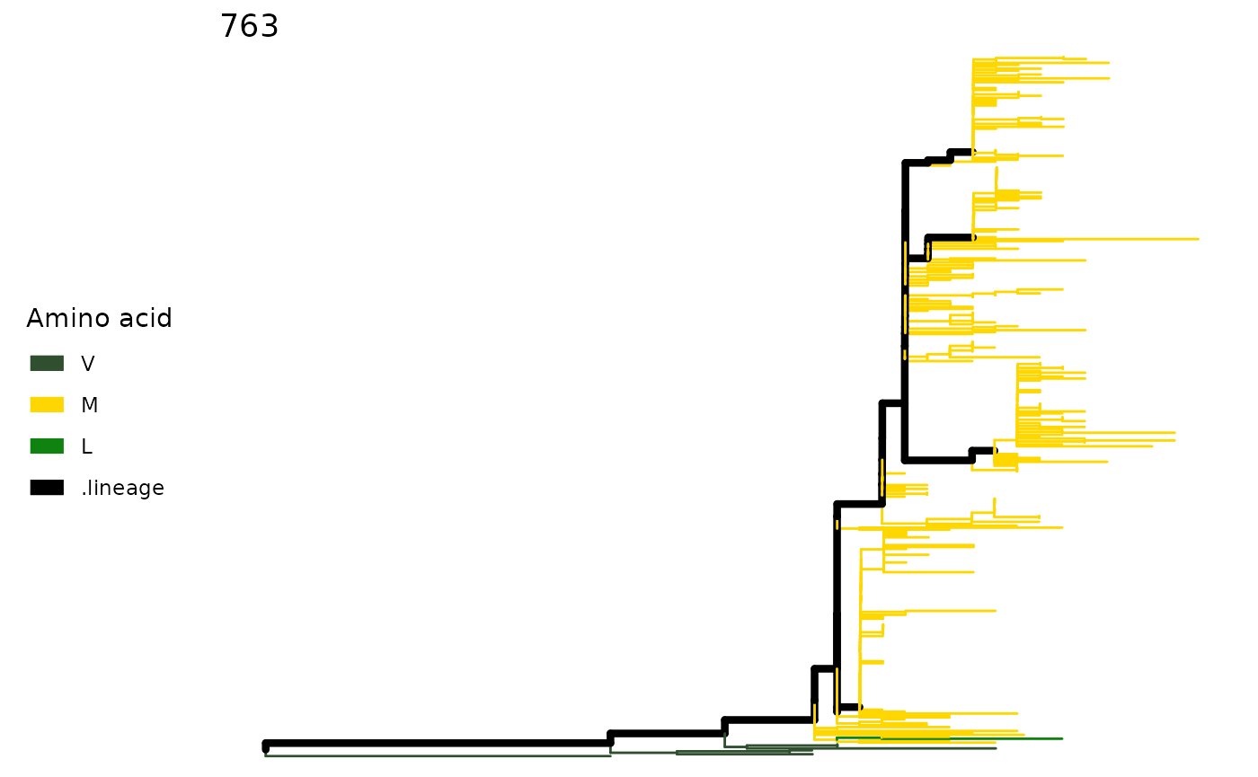
SNP sites
An SNP site could potentially undergo fixation event. The
SNPsites function predicts possible SNP sites and the
result could be what you’ll expect to be fixation mutation. Also, a tree
plot with mutation could be visualized with plotMutSites
function.
snps <- SNPsites(paths)
plotMutSites(snps)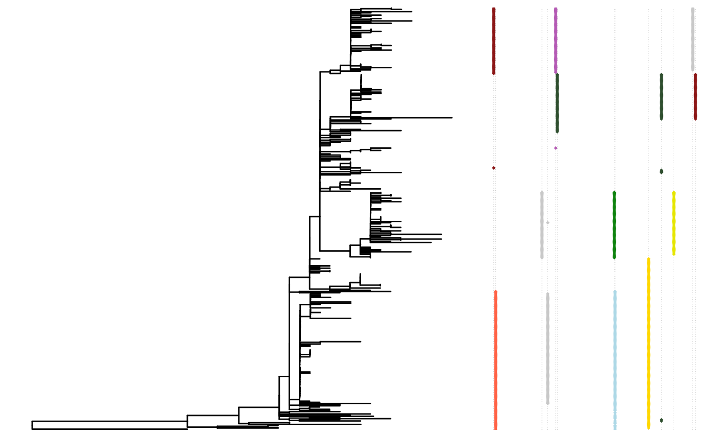
plotSingleSite(paths, snps[4])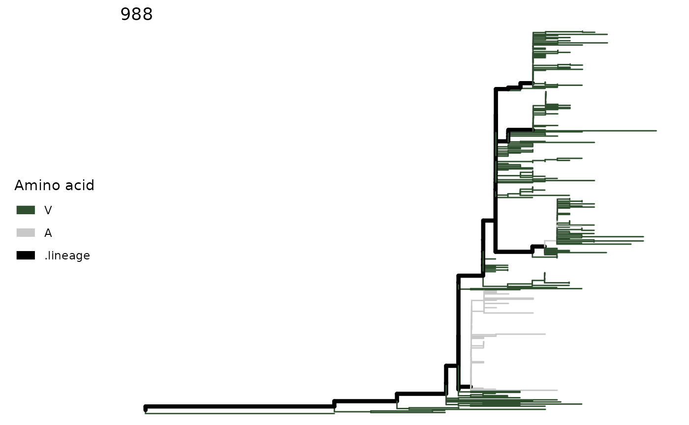
plotSingleSite(paths, snps[5])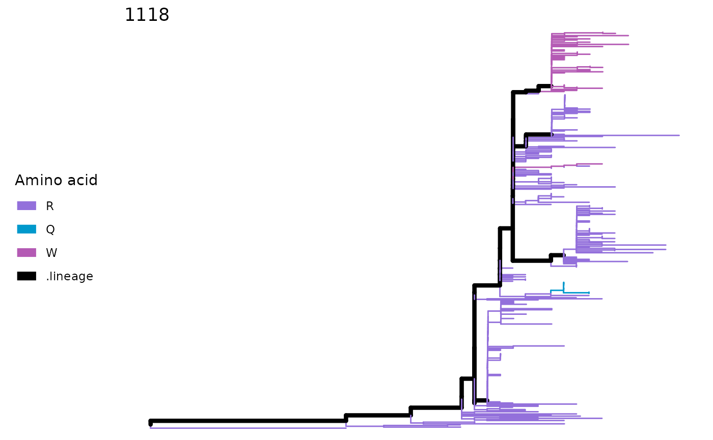
Session info
sessionInfo()
#> R version 4.2.1 (2022-06-23)
#> Platform: x86_64-pc-linux-gnu (64-bit)
#> Running under: Ubuntu 20.04.5 LTS
#>
#> Matrix products: default
#> BLAS:   /usr/lib/x86_64-linux-gnu/openblas-pthread/libblas.so.3
#> LAPACK: /usr/lib/x86_64-linux-gnu/openblas-pthread/liblapack.so.3
#>
#> locale:
#>  [1] LC_CTYPE=en_US.UTF-8       LC_NUMERIC=C
#>  [3] LC_TIME=en_US.UTF-8        LC_COLLATE=en_US.UTF-8
#>  [5] LC_MONETARY=en_US.UTF-8    LC_MESSAGES=en_US.UTF-8
#>  [7] LC_PAPER=en_US.UTF-8       LC_NAME=C
#>  [9] LC_ADDRESS=C               LC_TELEPHONE=C
#> [11] LC_MEASUREMENT=en_US.UTF-8 LC_IDENTIFICATION=C
#>
#> attached base packages:
#> [1] stats     graphics  grDevices utils     datasets  methods   base
#>
#> other attached packages:
#> [1] sitePath_1.13.0  BiocStyle_2.25.0
#>
#> loaded via a namespace (and not attached):
#>  [1] ggrepel_0.9.1       Rcpp_1.0.9          ape_5.6-2
#>  [4] lattice_0.20-45     tidyr_1.2.0         rprojroot_2.0.3
#>  [7] digest_0.6.29       utf8_1.2.2          R6_2.5.1
#> [10] evaluate_0.16       highr_0.9           ggplot2_3.3.6
#> [13] pillar_1.8.1        ggfun_0.0.7         yulab.utils_0.0.5
#> [16] rlang_1.0.5         lazyeval_0.2.2      rstudioapi_0.14
#> [19] jquerylib_0.1.4     rmarkdown_2.16      pkgdown_2.0.6
#> [22] labeling_0.4.2      textshaping_0.3.6   desc_1.4.2
#> [25] stringr_1.4.1       munsell_0.5.0       compiler_4.2.1
#> [28] xfun_0.33           pkgconfig_2.0.3     systemfonts_1.0.4
#> [31] gridGraphics_0.5-1  htmltools_0.5.3     tidyselect_1.1.2
#> [34] gridExtra_2.3       tibble_3.1.8        bookdown_0.29
#> [37] fansi_1.0.3         dplyr_1.0.9         MASS_7.3-58.1
#> [40] grid_4.2.1          nlme_3.1-159        jsonlite_1.8.0
#> [43] gtable_0.3.1        lifecycle_1.0.2     magrittr_2.0.3
#> [46] scales_1.2.1        tidytree_0.4.0      cli_3.4.0
#> [49] stringi_1.7.8       cachem_1.0.6        farver_2.1.1
#> [52] fs_1.5.2            ggtree_3.5.3        seqinr_4.2-16
#> [55] bslib_0.4.0         ragg_1.2.2          generics_0.1.2
#> [58] vctrs_0.4.1         RColorBrewer_1.1-3  tools_4.2.1
#> [61] treeio_1.21.2       ade4_1.7-19         ggplotify_0.1.0
#> [64] glue_1.6.2          purrr_0.3.4         parallel_4.2.1
#> [67] fastmap_1.1.0       yaml_2.3.5          colorspace_2.0-3
#> [70] BiocManager_1.30.18 aplot_0.1.7         memoise_2.0.1
#> [73] knitr_1.40          patchwork_1.1.2     sass_0.4.2